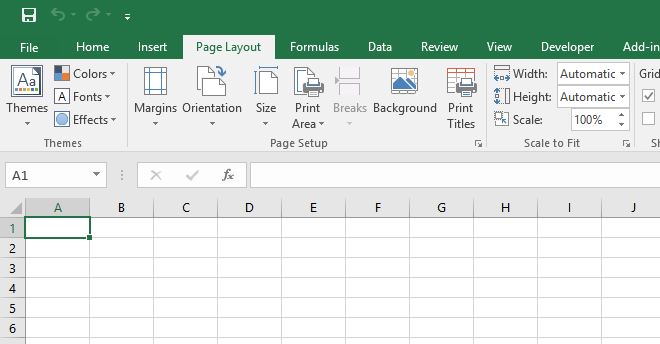
Microsoft Excel ribbon is the row of tabs and icons at the top of the Excel window that allows you to quickly find, understand and use commands for completing a certain task. The ribbons in Excel is made up of four basic components: tabs, groups, dialog launchers, and command buttons.
Excel ribbon is the row of tabs and icons at the top of the Excel window that allows you to find, understand and use commands for completing a certain task. Excel ribbon is the primary interface that contains every command and feature. The Ribbon has multiple display options according to your preferences.
In Excel Ribbons, the buttons and icons are grouped into different tabs based on the category of their functionalities. It contains seven tabs: Home, Insert, Page Layout, Formulas, Data, Review, and View.
The Ribbon first appeared in Excel 2007, replacing the traditional toolbars and pull-down menus found in previous versions. In Excel 2010, Microsoft added the ability to personalize the Ribbon.
Tabs
The tabs on the ribbon are: File, Home, Insert, Page layout, Formulas, Data, Review, View Developer & Add-ins. The Home tab contains the most frequently used commands in Excel.

Groups
Each tab contains groups of related commands. For example, the Page Layout tab contains the Themes group, the Page Setup group, etc.

Use the Ribbon
Let’s use the ribbon to insert a table. Tables allow you to analyze your data in Excel quickly and easily.
1. Click any single cell inside a data set.
2. On the Insert tab, in the Tables group, click Table.

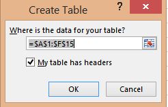
3. Excel automatically selects the data for you. Check ‘My table has headers’ and click on OK.

Result. Excel creates a nicely formatted table for you.

Note: use the drop-down arrows to quickly sort and filter. Visit our chapter about tables to learn more about this topic.
Collapse the Ribbon
You can collapse the ribbon to get extra space on the screen. Right click anywhere on the ribbon, and then click Collapse the Ribbon (or press + ).

Result.

