Named Range
Create a named range or a named constant and use these names in your Excel formulas. This way you can make your formulas easier to understand.
To create a named range, execute the following steps.
1. Select the range A1:A4.

2. On the Formulas tab, in the Defined Names group, click Define Name.

3. Enter a name and click OK.

There’s an even quicker way of doing this.
4. Select the range, type the name in the Name box and press Enter.

5. Now you can use this named range in your formulas. For example, sum Prices.

To create a named constant, execute the following steps.
6. On the Formulas tab, in the Defined Names group, click Define Name.

7. Enter a name, type a value, and click OK.

8. Now you can use this named constant in your formulas.

If the tax rate changes, use the Name Manager to edit the value and Excel automatically updates all the formulas that use TaxRate.
9. On the Formulas tab, in the Defined Names group, click Name Manager.

10. Select TaxRate and click Edit.

Note: use the Name Manager to view, create, edit and delete named ranges.
If your data has labels, you can quickly create named ranges in Excel.
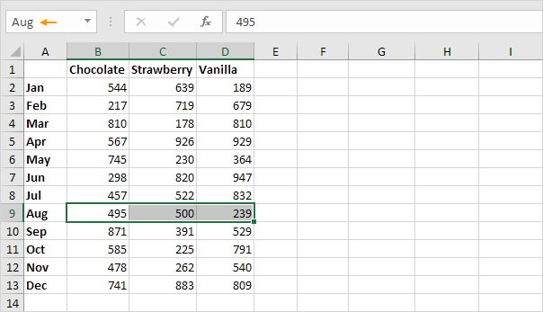
11. For example, select the range A1:D13.

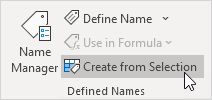
12. On the Formulas tab, in the Defined Names group, click Create from Selection.

13. Check Top row and Left column and click OK.

14. Excel created 12 + 3 = 15 named ranges! Simply select a range and look at the Name box.

15. Use the intersect operator (space) to return the intersection of two named ranges.

Note: try it yourself. Download the Excel file, create the named ranges quickly and easily (start with step 11) and lookup any value in this two-dimensional range.