Master Excel basics by learning how to format cells, adjust alignment, apply borders, and customize number formats to improve your spreadsheet’s appearance.
Introduction to Format Cells
When we format cells in Excel, we change the appearance of a number without changing the number itself. We can apply a number format (0.5, $0.50, 50%, etc) or other formatting (alignment, font, border, etc).
1. Enter the value 0.5 into cell B4.
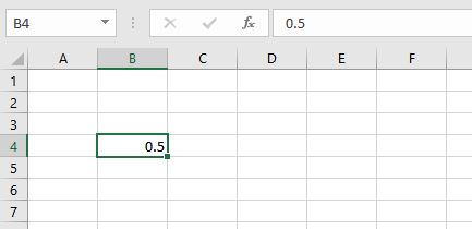
By default, Excel uses the General format (no specific number format) for numbers. To apply a number format, use the ‘Format Cells’ dialog box.
2. Select cell B4.
3. Right click, and then click Format Cells (or press + ).
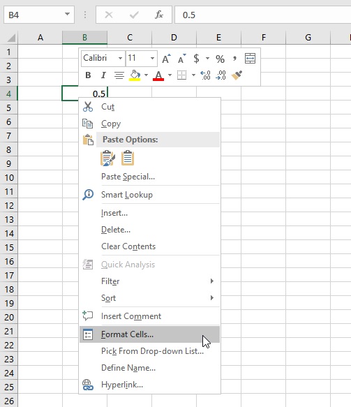
The ‘Format Cells’ dialog box appears.
4. For example, select Currency.

Note: Excel gives you a life preview of how the number will be formatted (under Sample).
5. Click OK.

Cell B4 still contains the number 0.5. We only changed the appearance of this number. The most frequently used formatting commands are available on the Home tab.
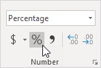
6. On the Home tab, in the Number group, click the percentage symbol to apply a Percentage format.
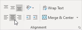
7. On the Home tab, in the Alignment group, center the number.
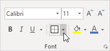
8. On the Home tab, in the Font group, add outside borders and change the font color to Red.
Result:

Conclusion
You can also use the Format Cell dialog box to formatting cell. To open the Format Cell dialog box, select the cells you want to format and then click on the Format button in the Number group on the Home tab.
The Format Cell dialog box has a variety of formatting options, including:
- Number formatting: You can choose a number format to display numbers in a variety of ways, such as as currency, dates, or percentages.
- Alignment: You can choose an alignment option to control how text is aligned in a cell.
- Font: You can choose a font, font size, and font color for the text in a cell.
- Border: You can choose a border style to add borders to a cell.
- Fill: You can choose a fill color to fill a cell with a color.
| Next Chapter: Find & Select |