A pivot tables are the powerful tool in Excel that allows you to summarize and analyze large amounts of data. It is a dynamic tool, meaning that you can easily change the way the data is summarized by dragging and dropping fields in the pivot table.
Introduction
Pivot tables are often used to answer questions about data. For example, you could use a pivot table to answer the following questions:
- What are the top 5 products sold by month?
- The average sales by salesperson?
- What are the sales trends over time?
Pivot tables can be used to summarize data in a variety of ways. You can summarize data by:
- Sum: This is the most common type of summary. It simply adds up all the values in a field.
- Count: This counts the number of items in a field.
- Average: This calculates the average value of a field.
- Max: This returns the maximum value in a field.
- Min: This returns the minimum value in a field.
You can also create custom summaries by using calculated fields. Calculated fields are formulas that you create to summarize data in a specific way. For example, you could create a calculated field that calculates the total sales for each salesperson, minus the cost of goods sold.
Example
Our data set consists of 213 records and 6 fields. Order ID, Product, Category, Amount, Date and Country.

Insert a Pivot Table
To insert a pivot table, execute the following steps.
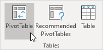
1. Click any single cell inside the data set.
2. On the Insert tab, in the Tables group, click PivotTable.
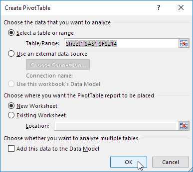
The following dialog box appears. Excel automatically selects the data for you. The default location for a new pivot table is New Worksheet.
3. Click OK.
Drag fields
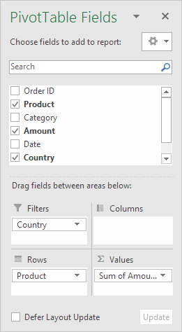
The PivotTable Fields pane appears. To get the total amount exported of each product, drag the following fields to the different areas.
1. Product field to the Rows area.
2. Amount field to the Values area.
3. Country field to the Filters area.
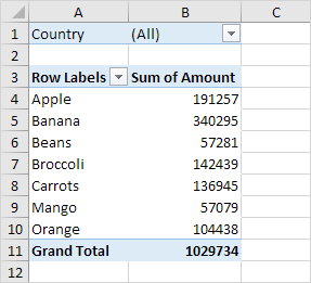
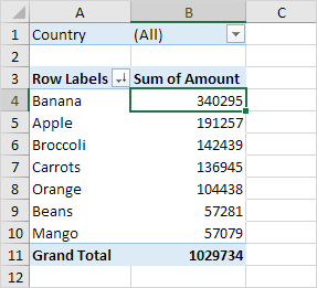
Below you can find the pivot table. Bananas are our main export product. That’s how easy pivot tables can be!
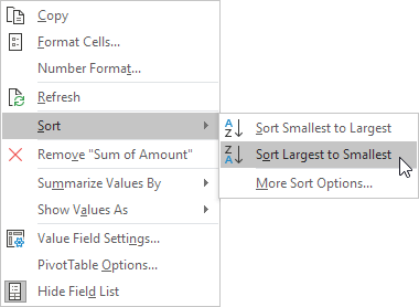
Sort
To get Banana at the top of the list, sort the pivot table.
1. Click any cell inside the Sum of Amount column.
2. Right click and click on Sort, Sort Largest to Smallest.
Result.
Filter
Because we added the Country field to the Filters area, we can filter this pivot table by Country. For example, which products do we export the most to France?
1. Click the filter drop-down and select France.
Result. Apples are our main export product to France.
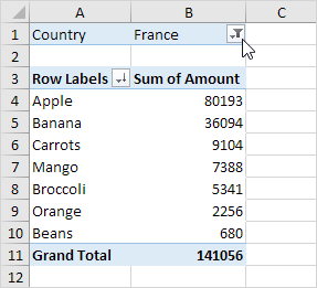
Note: you can use the standard filter (triangle next to Row Labels) to only show the amounts of specific products.
Change Summary Calculation
By default, Excel summarizes your data by either summing or counting the items. To change the type of calculation that you want to use, execute the following steps.
1. Click any cell inside the Sum of Amount column.
2. Right click and click on Value Field Settings.
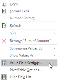
3. Choose the type of calculation you want to use. For example, click Count.
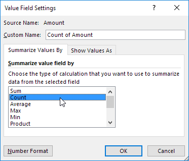
4. Click OK.
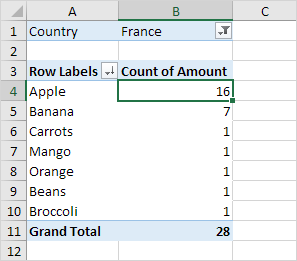
Result. 16 out of the 28 orders to France were ‘Apple’ orders.
Two-dimensional Pivot Table
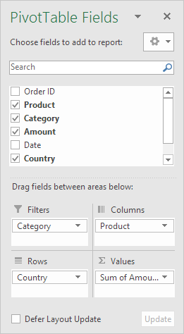
If you drag a field to the Rows area and Columns area, you can create a two-dimensional pivot table. First, insert a pivot table. Next, to get the total amount exported to each country, of each product, drag the following fields to the different areas.
1. Country field to the Rows area.
2. Product field to the Columns area.
3. Amount field to the Values area.
4. Category field to the Filters area.
Below you can find the two-dimensional pivot table.
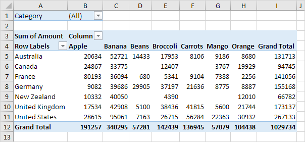
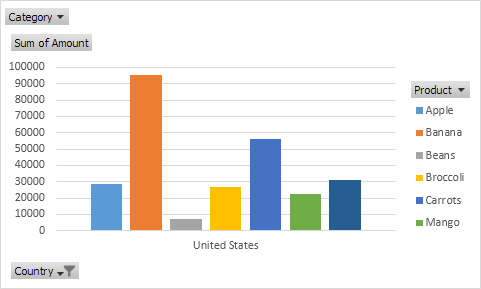
To easily compare these numbers, create a pivot chart and apply a filter. Maybe this is one step too far for you at this stage, but it shows you one of the many other powerful pivot table features Excel has to offer.
Pivot tables are a powerful tool for data analysis. They are easy to use and can be used to summarize data in a variety of ways. If you are working with large amounts of data, pivot tables are a valuable tool that you should learn to use.
Benefits of Pivot Tables
Here are some of the benefits of using pivot tables:
- They can help you to summarize large amounts of data quickly and easily.
- You to identify trends and patterns in your data with the help of Pivot tables.
- They can help you to answer specific questions about your data.
- They are dynamic, meaning that you can easily change the way the data is summarized.
- They can be used to create charts and graphs.
Limitations of Pivot Tables
Here are some of the limitations of using pivot tables:
- Difficult to learn how to use.
- They can be slow to calculate if you have a lot of data.
- They can be difficult to troubleshoot if something goes wrong.
Overall, pivot tables powerfully summarize and analyze large amounts of data. They are easy to use and can answer specific questions about your data. However, they can be difficult to learn how to use and can be slow to calculate if you have a lot of data.
| Next Chapter: Tables |