Excel Functions – Formula Errors in Excel

Introduction

This chapter teaches you how to deal with some common formula errors in Excel. Let’s start simple.

#####

When your cell contains this error code, the column isn’t wide enough to display the value.

1. Click on the right border of the column A header and increase the column width.

Tip: double click the right border of the column A header to automatically fit the widest entry in column A.

#NAME?

The #NAME? error occurs when Excel does not recognize text in a formula.

1. Simply correct SU to SUM.

#VALUE!

Excel displays the #VALUE! error when a formula has the wrong type of argument.

1a. Change the value of cell A3 to a number.
1b. Use a function to ignore cells that contain text.

#DIV/0!

Excel displays the #DIV/0! error when a formula tries to divide a number by 0 or an empty cell.

1a. Change the value of cell A2 to a value that is not equal to 0.
1b. Prevent the error from being displayed by using the logical function IF.

Explanation: if cell A2 equals 0, an empty string (“) is displayed. If not, the result of the formula A1/A2 is displayed.

#REF!

Excel displays the #REF! error when a formula refers to a cell that is not valid.

1. Cell C1 references cell A1 and cell B1.

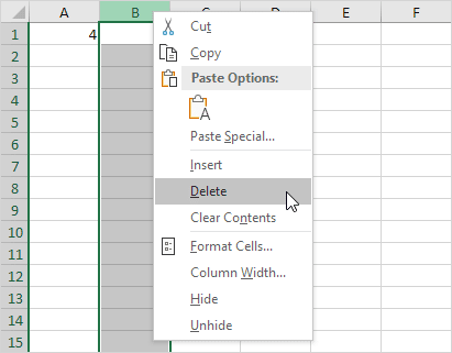
2. Delete column B. To achieve this, right click the column B header and click Delete.

3. Select cell B1. The reference to cell B1 is not valid anymore.

4. To fix this error, you can either delete +#REF! in the formula of cell B1 or you can undo your action by pressing CTRL + z

The #N/A error appears when the VLOOKUP function (or XLOOKUP, MATCH, etc.) can’t find a match.

1. In the example below, ID 28 cannot be found.

2. Use the IFNA function to replace the #N/A error with a friendly message.

#NUM!

Excel shows the #NUM! error when a formula contains invalid numeric values.

1. For example, the SQRT function below cannot calculate the square root of a negative number.

2. Change the number in cell A1 to a positive number.

#NULL!

The intersect operator (single space) returns the intersection of two ranges. When two ranges don’t intersect, Excel displays the #NULL! error.

1. The formula below returns #NULL! because the two ranges don’t intersect.

2. The formula below doesn’t return the #NULL error.

Note: =SUM(F2:G2) produces the exact same result!

#SPILL!

If something is blocking a spill range, Excel displays the #SPILL! error.

1. Simply empty cell C6 to fix the #SPILL error.

Note: this dynamic array function, entered into cell C1, fills multiple cells. Wow! This behavior in Excel 365/2021 is called spilling.

Tips

If you see one of these error codes, the first step is to troubleshoot the problem. Here are some tips for troubleshooting Excel formula errors:

• Check your spelling. Formulas are case-sensitive, so make sure you’ve spelled all of the function names and cell references correctly.
• Check your data types. Make sure that the values in your cells are the correct data types for the functions you’re using.
• Check your cell references. Make sure that the cells you’re referencing actually exist.
• Check for circular references. A circular reference occurs when a formula refers to itself. This can cause Excel to give inaccurate results or stop working altogether.

If you’ve checked all of these things and you’re still getting an error, you can use the ERROR.TYPE function to find out more information about the error. The ERROR.TYPE function returns a number that represents the type of error that occurred. You can then use this number to look up the error message in the Excel help file.

Once you’ve identified the cause of the error, you can fix it and your formula should start working correctly.

Avoiding Formula Errors

The best way to avoid formula errors is to be careful when you’re creating and editing formulas. Here are some tips for avoiding formula errors:

• Formula Auditing is useful tool to find and fix errors.
• Use the IFERROR function to trap and handle errors.
• Use the ERROR.TYPE function to get more information about errors.
• Back up your work regularly so that you can recover from errors.

By following these tips, you can help to ensure that your Excel formulas are accurate and error-free.